
Is a 10% annual return impressive, or is it simply the reward for taking a lot of risk? The Sharpe ratio answers that question with one number: how much return a portfolio earned above a risk-free investment for each unit of volatility it went through. Here is the Sharpe ratio explained step by step: the formula, a worked example with monthly returns, how to annualize the result, what counts as a good value and where the ratio can mislead you.
Sharpe ratio explained: meaning and origin
The Sharpe ratio is one of the most widely quoted measures of risk-adjusted performance. It was introduced by William F. Sharpe in 1966, in a study of mutual fund performance, under the name “reward-to-variability ratio”. Sharpe, who shared the 1990 Nobel Memorial Prize in Economic Sciences with Harry Markowitz and Merton Miller, revisited and generalized the measure in a 1994 article titled “The Sharpe Ratio”.
Raw returns are not comparable when the risks behind them differ. The Sharpe ratio puts every portfolio on the same footing by dividing its excess return (the return above a risk-free rate) by its volatility. A higher ratio means more excess return per unit of volatility. It is widely used to compare mutual funds, ETFs and fund managers. It helps you answer three practical questions:
- Were an investment’s returns worth the swings you had to sit through?
- How did a portfolio do compared with simply holding a risk-free asset?
- Of two portfolios with similar returns, which one got there more efficiently?
The Sharpe ratio formula
Sharpe ratio = (Rp − Rf) / σp
- Rp: the average return of the portfolio over the period studied.
- Rf: the risk-free rate over the same period, usually a short-term government bill yield.
- σp: the standard deviation of the portfolio’s returns, in other words its volatility.
Strictly speaking, Sharpe’s 1994 definition divides the average excess return by the standard deviation of the excess returns (portfolio return minus risk-free return, period by period). When the risk-free rate barely moves over the period, the two standard deviations are almost identical, which is why most calculators simply use the volatility of the portfolio.
Historical (ex-post) versus expected (ex-ante)
Most Sharpe ratios you see are ex-post: they are calculated from realized past returns. An ex-ante Sharpe ratio uses expected returns and expected volatility instead, for example when comparing portfolio allocations in a model. Both use the same formula. An ex-post ratio describes the past, not the future, and an ex-ante ratio is only as reliable as the forecasts behind it.
Which risk-free rate should you use?
Use a short-term rate in the same currency as the returns and for the same period: US Treasury bills for a portfolio measured in dollars, a short-term euro rate such as €STR or short-dated government bills for a portfolio measured in euros. Convert it to the frequency of your data. An annual rate of 3.6% becomes 0.30% per month (a simple division by 12 is the usual convention for this step).
How to calculate the Sharpe ratio: a worked example
Take a hypothetical balanced portfolio with the following 12 monthly returns, and a risk-free rate of 3.6% a year, or 0.30% a month. The numbers are illustrative only.
| Month | Return | Month | Return |
|---|---|---|---|
| 1 | +2.1% | 7 | +2.4% |
| 2 | −1.4% | 8 | −0.7% |
| 3 | +3.0% | 9 | +1.2% |
| 4 | +0.8% | 10 | −3.1% |
| 5 | −2.6% | 11 | +4.0% |
| 6 | +1.9% | 12 | +1.5% |
- Average monthly return. The 12 returns add up to 9.1%, so the arithmetic mean is 9.1 / 12 = 0.758% per month.
- Average monthly excess return. 0.758% − 0.30% = 0.458% per month.
- Volatility. The sample standard deviation of the monthly returns (STDEV.S in Excel) is 2.237%. Because the risk-free rate is constant here, the excess returns have exactly the same standard deviation.
- Monthly Sharpe ratio. 0.458 / 2.237 = 0.205.
- Annualized Sharpe ratio. 0.205 × √12 = 0.205 × 3.464 = 0.71.
You reach the same answer by annualizing each part first: the mean excess return becomes 0.458% × 12 = 5.5% a year, volatility becomes 2.237% × √12 = 7.75% a year, and 5.5 / 7.75 = 0.71. If you only have annual figures, the shortcut is the same formula: a portfolio that returned 9% with 15% volatility while bills paid 3% has a Sharpe ratio of (9 − 3) / 15 = 0.40.
One detail matters here: the standard calculation uses the arithmetic average of the periodic returns, not the compounded return. Compounding the same 12 months gives about 9.19%, against 9.1% for twelve times the monthly average, and mixing the two methods across funds makes comparisons less reliable.
How to annualize the Sharpe ratio
Sharpe ratios are normally quoted on an annual basis, so ratios computed from monthly, weekly or daily data are scaled up. The average return grows in proportion to the number of periods, while the standard deviation grows only with the square root of that number. The ratio therefore scales with the square root of the number of periods per year:
| Data frequency | Periods per year | Multiply the periodic Sharpe ratio by |
|---|---|---|
| Monthly | 12 | √12 ≈ 3.46 |
| Weekly | 52 | √52 ≈ 7.21 |
| Daily (trading days) | 252 | √252 ≈ 15.87 |
A daily Sharpe ratio of 0.05, for example, annualizes to 0.05 × 15.87 ≈ 0.79. This square-root rule assumes returns are independent from one period to the next. When returns are autocorrelated, which is common for assets priced with a lag or smoothed by appraisals, the rule can overstate or understate the true annual figure; Andrew Lo’s 2002 paper “The Statistics of Sharpe Ratios” discusses the correction.
Comparing two portfolios with the Sharpe ratio
| Portfolio | Annual return | Volatility | Sharpe ratio (Rf = 2%) |
|---|---|---|---|
| A | 12% | 10% | (12 − 2) / 10 = 1.00 |
| B | 15% | 20% | (15 − 2) / 20 = 0.65 |
Portfolio B has the higher return, but Portfolio A earned more excess return per unit of volatility. In textbook portfolio theory this is what makes A more efficient: if you could borrow at the risk-free rate and hold A at twice its size, you would get 2 × 12% − 2% = 22% with 20% volatility, still a Sharpe ratio of 1.00, and more return than B for the same volatility. In practice, borrowing costs more than the risk-free rate and leverage brings risks that volatility does not capture, such as margin calls and deeper drawdowns. The comparison is a way to read efficiency, not a reason to borrow.
What is a good Sharpe ratio?
You will often see the following rules of thumb for annualized Sharpe ratios. They are conventions, not standards, and they say nothing about the future.
| Annualized Sharpe ratio | How it is often described | What to keep in mind |
|---|---|---|
| Below 0 | Return below the risk-free rate | The ratio becomes hard to rank (see limits below) |
| 0 to 1 | Positive but modest | Normal for many long-only stock and balanced portfolios over long periods |
| 1 to 2 | Good | Is the period long enough, and does it include a market downturn? |
| 2 to 3 | Very good | Smoothed prices, short history, survivorship bias, costs left out |
| Above 3 | Excellent on paper | Backtest overfitting or hidden tail risk are frequent explanations |
Context matters more than the label. Measured on long runs of annual data, a broad US stock index has typically shown a Sharpe ratio of roughly 0.3 to 0.5, so a long-only stock portfolio that sustains well above 1 over decades is unusual. Shorter windows can show much higher figures: three calm, rising years can push a fund’s ratio above 1.5, and a single bear market can turn it negative. A good Sharpe ratio is therefore one that compares favorably with similar portfolios measured over the same period, frequency, currency and risk-free rate, and that still holds up once a full market cycle is included.
Limits of the Sharpe ratio
- Upside and downside count the same. Standard deviation treats a sharp gain as risk, just like a sharp loss. If downside risk is what you care about, the Sortino vs Sharpe comparison shows how the Sortino ratio uses only downside deviation.
- Fat tails and skew are invisible. Standard deviation describes returns well only when they are roughly bell-shaped. Strategies that earn small, steady gains and occasionally suffer a large loss, such as selling options, can show a high Sharpe ratio until the loss arrives.
- Smoothed returns flatter the ratio. Assets valued by appraisal or traded rarely show artificially low volatility, which inflates their Sharpe ratio.
- The estimate is noisy. Under simple assumptions, a Sharpe ratio of 0.5 measured on ten years of monthly returns has a standard error of roughly 0.3. Small differences between two funds are often statistical noise.
- Negative ratios rank badly. When the excess return is negative, more volatility makes the ratio less negative. A fund 2% below the risk-free rate with 20% volatility scores −0.10, which looks better than a fund with the same shortfall and only 10% volatility (−0.20).
- Total risk is not always the right risk. For a single holding inside a diversified portfolio, much of its volatility is diversified away. The Treynor ratio divides excess return by beta, a measure of the market risk that diversification cannot remove.
- The path is ignored. Two portfolios with the same Sharpe ratio can have very different worst peak-to-trough losses. Pair it with maximum drawdown to see how deep the losses went.
- It says nothing about price. A stock with a strong trailing Sharpe ratio can still be expensive relative to its fundamentals. Valuation is a separate question; our research methodology explains how valuation, quality, growth, risk and technical context are weighed when prioritizing stocks to study.
Sharpe ratio versus other risk-adjusted measures
| Measure | Formula | Risk in the denominator | Typical use |
|---|---|---|---|
| Sharpe ratio | (Rp − Rf) / σp | Total volatility | Comparing whole portfolios or funds |
| Sortino ratio | (Rp − target) / downside deviation | Volatility below a target | Asymmetric return profiles |
| Treynor ratio | (Rp − Rf) / βp | Market (systematic) risk | A holding within a diversified portfolio |
| Information ratio | (Rp − Rb) / tracking error | Deviation from a benchmark | Judging active managers |
| Calmar ratio | Annualized return / maximum drawdown | Worst peak-to-trough loss | Strategies where deep losses matter most |
Frequently asked questions
Is a Sharpe ratio of 1 good?
For an annualized figure, 1 is usually described as good, and over a full market cycle it is above what a broad stock index has typically delivered. Over a short or unusually calm period, it may say more about the period than about the portfolio.
Can the Sharpe ratio be negative?
Yes. A negative Sharpe ratio means the portfolio returned less than the risk-free rate over the period, so a risk-free asset would have done better. Be careful when ranking negative values, because higher volatility makes a negative ratio look less bad.
How do you annualize a Sharpe ratio from daily or monthly returns?
Multiply the periodic Sharpe ratio by the square root of the number of periods in a year: √12 for monthly data and √252 for daily data based on trading days. The rule assumes returns are independent from one period to the next.
How do you calculate the Sharpe ratio in Excel?
With 12 monthly returns in cells B2 to B13 entered as decimals and a monthly risk-free rate of 0.003, use =(AVERAGE(B2:B13)-0.003)/STDEV.S(B2:B13)*SQRT(12). With the returns from the worked example above, this returns about 0.71.
What is the Sharpe ratio of the S&P 500?
There is no single figure: it depends on the dates, the data frequency and the risk-free rate. Over long histories of annual data it has typically been around 0.3 to 0.5, while a single year or a three-year window can be well above 1 or below 0. Compare a fund with the index using the same inputs for both.
What is the difference between the Sharpe and Sortino ratios?
Both divide excess return by a measure of risk. The Sharpe ratio uses total volatility, so gains and losses both count as risk. The Sortino ratio uses only the volatility of returns below a target, which gives a different picture for portfolios whose returns are not symmetrical.
Educational content, not investment advice.

Duration & Modified Duration – Measuring Interest Rate Sensitivity
Introduction Interest rate risk is one of the most important financial risks facing investors, especially those holding bonds and other fixed-income assets. Understanding…

Contribution to Risk & Risk Budgeting – Managing Portfolio Fragility
Want to know which assets make your portfolio fragile? Explore how Contribution to Risk and Risk Budgeting can help you identify, measure, and control risk efficiently.
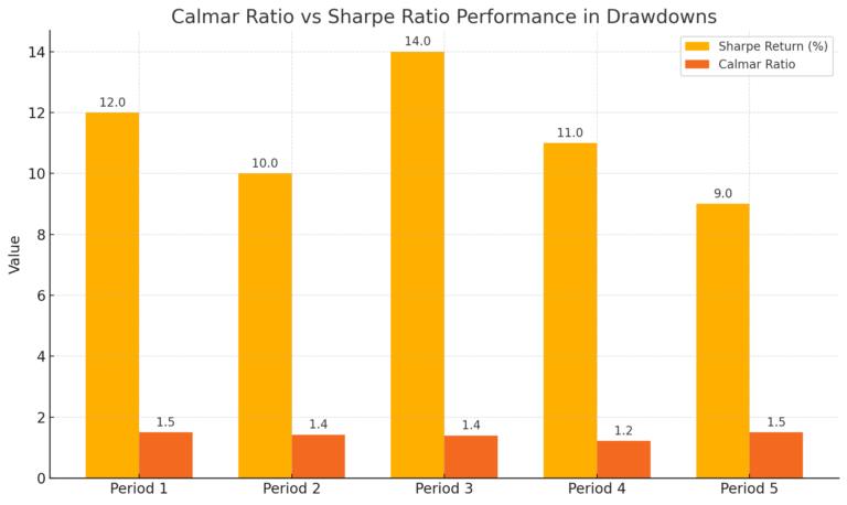
Calmar Ratio – A Better View of Risk in Volatile Times
The Calmar Ratio offers investors a clearer understanding of how well an investment performs relative to its worst drawdown. It’s a must-know for portfolio managers navig…
Go further
Turn the headlines into a watchlist
Compare valuation, quality and risk in the stock valuation scanner, then follow the alerts.
0 Comments